
Contours of Crisis: Plus ça change, plus c’est pareil?
First in a series of articles on the current crisis.
This is a web-only article from the website of Dollars & Sense: The Magazine of Economic Justice available at http://www.dollarsandsense.org
This is a web-only article, available only at www.dollarsandsense.org.
Subscribe Now
at a 30% discount.

This is the first in a series of short articles we plan to write on the current crisis. Our aim in this series is threefold: to outline some of the important contours of the crisis; to situate these patterns in historical context; and to reflect on their possible causes and implications.
Since the crisis is still ongoing, such analysis can only be cursory and suggestive. But it is nonetheless useful to put our preliminary research and thoughts in writing. By spelling out what we do know (or think we know) about the crisis, we can better identify what we don’t know and need to ask.
This paper sets the stage for the series. It outlines the conventional wisdom about the cause of crisis; it describes the chronology of events; and it contrasts the pattern and magnitude of the current downturn with those of earlier episodes. The overall picture painted by this analysis is highly stylized: crises appear to come and go with remarkable regularity, their oscillations are fairly similar and they share the same order of magnitude. The whole process seems almost “automatic,” and automaticity is reassuring: it suggests that the current crisis has run much of its course and that doom and gloom will soon give way to a new upswing.
But what if this automaticity is a mirage?
The Mismatch
Most observers like to blame the ongoing turbulence in the global political economy on finance—or more precisely, on a mismatch between finance and reality.
The mismatch begins with the assumption that there are two types of capital: “real” and “financial.” Real capital is a productive entity, made of machines, structures, work in progress and (some say) knowledge. Financial capital is a symbolic entity, consisting of equity and debt claims on real capital. In a perfect world, the two types of capital are exactly equal: the dollar value of GE’s stocks, bonds and other outstanding obligations represents the productive value of the company’s capital stock, so the two magnitudes must be the same. The assets and the entitlements to the assets have to match, by definition.
But the world isn’t perfect. Greed and fear, irrationality and fraud, corruption and manipulation, insufficient competition and too much government, overregulation and excessive deregulation, imperfect information and short-term memory, all conspire to distort the picture. These distortions cause finance to deviate from its “fair value,” either up or down. And as the deviation grows larger, finance ceases to mirror reality. It becomes a “fiction.”
The current crisis, goes the argument, is the unavoidable consequence of such deviation. Since the 1980s, we are told, finance has inflated into a huge bubble, having risen far above the underlying stocks of real assets. But then, whatever goes up must come down. Since finance, in the final analysis, is merely the image of the real thing, at some point it has to shrink back to its “true” size. And that is exactly what we are now witnessing: a violent financial crisis that dispels the fiction and brings finance down to its “par value.”
The Excess Unwound
According to the mismatch thesis, the current turmoil started in the U.S. housing market. This was the epicenter. From here the tremor spread like a tidal wave: first to the entire U.S. FIRE sector (an acronym for “finance, insurance and real estate”), then to every financial market around the world, and finally to the so-called “real economy.” This domino sequence is listed in Table 1 and illustrated in Figures 1, 2, and 3.
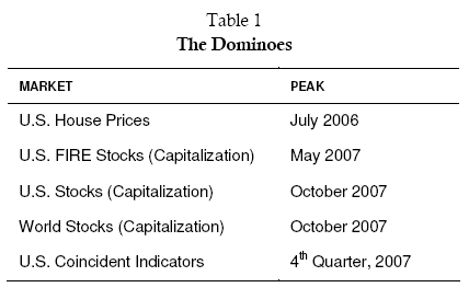
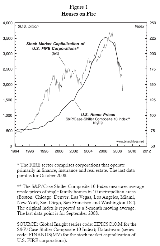
Figure 1 shows the rise and fall of U.S. house prices, along with the expansion and contraction of the FIRE sector. Prices of homes started to soar in 1997/8. According to the pundits, the blaze was fuelled by three key actors. The first was Fed Chairman and Ayn Rand acolyte Alan Greenspan, who lowered interest rates in the belief that “human nature” would limit risk taking. The second were the financial institutions that gladly ignored the risks and went on to offer mortgages to anyone willing to borrow. And the third were the eyes-wide-shut regulators, who seemed unable to see what was going on even if they cared. House prices had nowhere to go but up, and within a decade they tripled.
Everyone was bullish. Home buyers were eager to borrow, convinced that prices would go on rising and that their houses could always be resold at a profit. The bankers bent over backwards to lend them the money—and then melted the individual mortgages into large pools of asset-backed securities. And the so-called investment community—including “high net-worth individuals,” large corporations, money managers and the banks themselves—lined up to buy tranches of the new “structured investment vehicles,” usually without asking too many questions.
And for a while there was little to ask about. Since house prices were rising, default wasn’t an issue. A home owner who couldn’t service his mortgage would have his house repossessed and quickly resold to the next sucker in line, often at a higher price. And if the parties still felt that there was some residual risk left, they could always offset the hazard with higher interest rates, mortgage insurance and a whole slew of derivatives. The process seemed so robust that even “sub-prime” mortgages, lent to borrowers with little or no income, received a triple-A grading from honest-to-god analysts and fail-proof rating agencies.[Note 1]
By the early 2000s, the real-estate boom went global. Worldwide, the annual issuance of asset-back securities rose nearly five-fold—from $532 billion in 2000 to $2.5 trillion in 2006—with much of the expansion accounted for by mortgage-backed instruments, whose new issues rose from $275 billion in 2000 to over $2 trillion in 2006. In the United States, repackaging reached record levels. By the early 2000s, over half of all single home mortgages and roughly one third of multifamily home mortgages were melted and resold as securities—up from 10 and 5%, respectively, in 1980.[Note 2]
There was simply no way to lose money in this business, and the stock market certainly reflected that belief. The real-estate boom encouraged many other forms of debt financing, ranging from plain vanilla, to the exotic, to the kinky. And with U.S. FIRE companies cutting a profit on every deal, the total equity capitalization of their sector nearly quadrupled—from $1 trillion in 1997 to $3.7 trillion in 2007.
And then the music stopped.
As Figure 1 shows, in July 2006, U.S. house prices started to drop. Initially, investors hung in suspension. Pretending as if nothing had happened, they continued to buy FIRE stocks, pushing the market even higher. But the downward spiral in house prices persisted—and then, suddenly, in May 2007, everyone started rushing for the door. By September 2008, house prices were down nearly 25% relative to their 2006 peak, while U.S. FIRE stocks went into free fall. In October 2008, the total market capitalization of the sector was more than 50% below its May 2007 peak.
The gathering storm didn’t register immediately on the broader stock market. Figure 2 shows the market capitalization of three broad aggregates—U.S. FIRE equities, all U.S. equities, and all world equities. The three series are denominated in current $U.S. and plotted on a logarithmic scale to facilitate comparison.[Note 3]
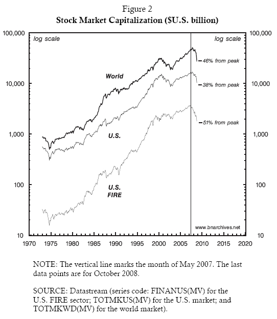
The data show that, while the U.S. FIRE sector started to drop in May 2007 (marked by the vertical line in the chart), the overall U.S. and global stock markets took another five months before tanking. However, once the broad reversal started, the downward convergence was swift. From October 2007 to October 2008, U.S. listed corporations lost 38 per cent of their market capitalization, while the global market lost 46 percent.
The last to join the downward spiral was the so-called “real economy.” Figure 3 shows the U.S. Composite Index of Coincident Indicators, a weighted average of four indicators that move more or less together with the business cycle.[Note 4] Although this Composite Index pertains only to the United States, in the current environment of global integration it provides a good proxy for world trends.
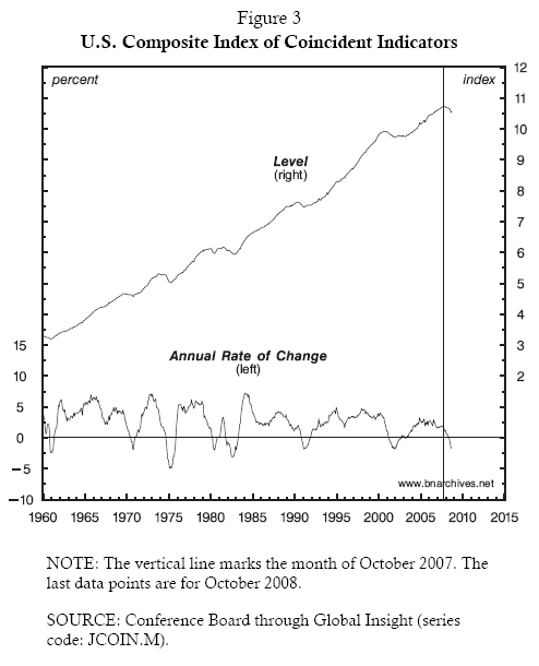
The figure presents two manifestations of the index: one is the actual level; the other is the annual rate of change, calculated by comparing the same month in successive years (so that the reading for October 2008 denotes the rate of change from October 2007, etc.). The growth series, plotted at the bottom of the chart, shows that the “real economy” started to decelerate at the end of 2006. But the actual level of the index, depicted by the top series, peaked at the end of 2007 (marked by the vertical line in the figure) and started its month-to-month declines only in early 2008.
So on the face of it, the world appears to be in the midst of a finance-led crisis, a decline triggered and significantly amplified by the collapse of fictitious capital. “The salient feature of the current financial crisis,” explains George Soros, “is that it was not caused by some external shock. ... The crisis was generated by the financial system itself.”[Note 5] According to this view, the biggest distortion was in the U.S. housing sector, whose bubble was the largest and first to deflate. The next victim was the broader financial market, which was also grossly inflated and therefore justly punctured. And the last to capitulate was the “real economy,” whose excesses obviously were more limited yet certainly worthy of a periodic cleanup.
But that is only half the story.
Toward a New Upswing?
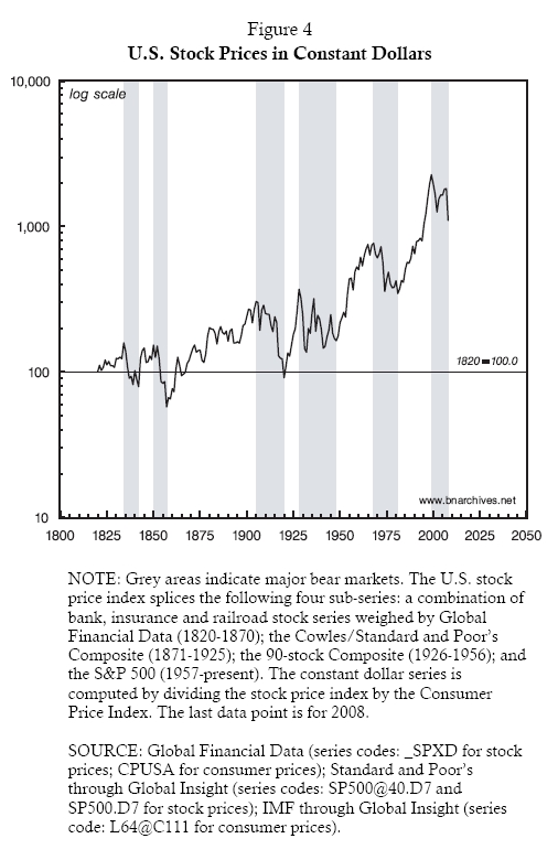
The mismatch thesis tells us that fictitious capital, by its very nature, tends to distort the picture in both directions: it grows by too much in the upswing, only to shrink by too much in the downswing. And indeed, many experts are already wondering if finance hasn’t been overly deflated.Measured against the historical record, the current market collapse certainly is extremely large. The magnitude of this collapse is contextualized in Figure 4 and Figure 5, where we show the history of U.S. stock prices since 1820. Before examining these charts, though, note that they express stock prices not in actual dollars, but in constant dollars. The latter measure is computed by dividing actual stock prices (expressed as an index) by consumer prices (also expressed as an index). This computation serves to “purge” from the stock market index the effect of inflation (and occasionally deflation). And once inflation has been expunged, the result represents stock prices denominated in constant dollars—i.e., in dollars with a “constant purchasing power.”[Note 6]
Why is it so important to distinguish between the two measures? To answer this question, note that stock prices in actual dollars can always be expressed as the product of two separate magnitudes: (1) the average price level of all commodities (in actual dollars), and (2) the ratio between stock prices and the average price level (which yields a pure number). This decomposition is true by definition:
Now, during periods of inflation or deflation, changes in the average price level (the first component on the right-hand side of the equation), can easily overwhelm changes that are unique to the stock market (the second component on the right). To illustrate, between 1900 and 2008, actual stock prices rose 133-fold. In terms of our equation, most of this increase was due to inflation: the average price level rose nearly 30-fold, whereas the ratio of stock prices to the average price level rose less than fivefold.[Note 7]
Clearly, stock owners are focused primarily on the second component. At the very minimum, their concern is not to keep up with inflation but to outperform it, and that is why we gauge the long-term performance of the stock market in constant dollars rather than actual ones.[Note 8]
With this qualification in mind, let us return now to Figure 4. The chart shows the stock market index in constant prices, plotted against a logarithmic scale. The vertical grey bars indicate what we consider to be major bear markets—i.e., periods during which the stock market suffered protracted declines.
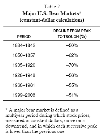
As it turns out, there is no general definition for a bear market—let alone a “major” one. So we’ve devised our own. In what follows we define a major bear market as a multiyear period during which stock prices, measured in constant dollars, move on a downtrend, and in which each successive peak is lower than the previous one. According to this definition, over the past two centuries, the United States experienced six major bear markets. These periods are listed in Table 2, along with the cumulative declines in stock prices.
A similar picture emerges from Figure 5, which measures the annual growth rate of the stock market index (again, in constant dollars). The thin line in the chart shows the percent variation from year to year. The thick line smoothes these variations as a 10-year moving average—meaning that every observation in the series measures the average annual growth rate in the previous ten years.[Note 9]
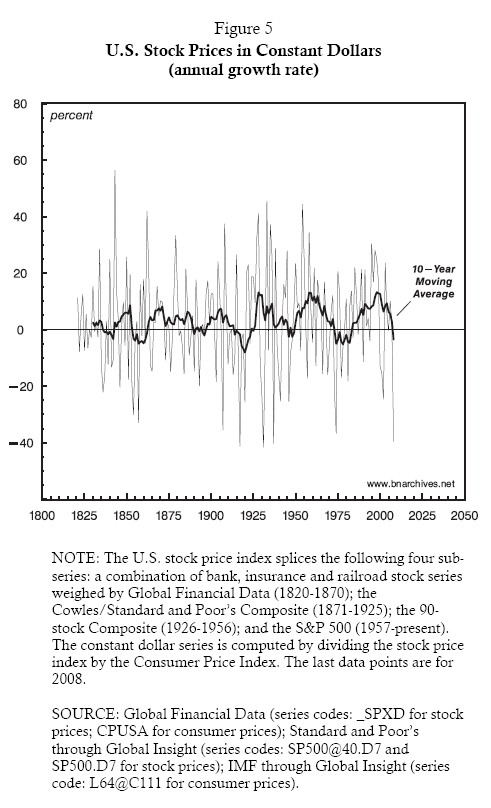
The last data points in Figure 5 are for 2008. The year-to-year change shows a drop of 40%—on par with the record declines of 1917, 1931, 1937 and 1974. Furthermore, as the moving-average series indicates and Figure 4 confirms, this decline wasn’t a fluke event, but rather part of a decade-long bear market. According to the smoothed series, the market peaked in 1998, with the 10-year moving average growth rate hovering around 13%. From then on, annual growth rates decelerated, and by 2008 pushed the 10-year moving average down to nearly –4%.
To the eyes of a seasoned financier, these magnitudes mean that the crisis may be approaching a bottom. According to Figure 5, prior crises were similarly bounded. Their highest starting point, measured by the 10-year moving average series, was 13% (in 1929 and in 1959), and their lowest trough, measured by the same series, was –8% (in 1920). The extent of deceleration in growth rates, measured by the peak-to-trough difference of the 10-year moving average, ranged from a low of 6.5% (during in the 1834-1842 crisis), to a high of 15.5% (in 1928-1948).
The present crisis, measured by the 10-year moving average series, has already met or exceeded these extreme values. It started from a record ceiling of 13.3%; its current low is –3.6%; and the extent of its deceleration, computed as the difference between these two values, marks a new record: 16.9%. For long-term investors, these numbers indicate that much of the crisis is probably behind them.
And the news gets even better. According to Figure 4, historically, each major bear market was followed by a long bull run, and each of those bull runs pushed stocks to a new record high. These upswings occurred in 1842–1850, 1857–1905, 1920–1928, 1948–1968 and 1981–1999, and it isn’t far fetched to think that a new one may soon be brewing.
Given that the present bear market is approaching historical lows, and since previously such bottoms were always followed by major upswings, many forward-looking strategists—from permanent bull Barton Biggs, to Wizard of Omaha Warren Buffet, to doom-and-gloom Martin Wolf—are now advising their followers to fasten their seat belts.[Note 10] News from the so-called “real economy” is likely to remain very bad and may possibly get worse—but most of the negatives are already “in the price.” And since fictitious capital is notorious for “overreacting,” particularly during deep downturns, current stock prices offer a once-in-a-life-time buying opportunity for those prescient enough to see into the next takeoff.
But, then, if the market has bottomed and the upswing is so certain, why isn’t every investor buying?
Financial Cycles and the Reordering of Society
It is easy to fall for the aesthetic gyrations of the stock market. Their stylized cycles make them look natural. They “revert to mean,” as Francis Galton would have it. They oscillate within fairly clear boundaries. Their ups and downs seem almost automatic (at least in retrospect). Their regularities are so neat many are tempted to forget David Hume and extrapolate the past into the future.
And here lies the problem. The long-term cycles of the stock market, no matter how stylized and regular they seem, are not self-generating. They don’t just happen on their own. Each cycle has a reason, and that reason is deeply social and historically unique.
Note that, during the twentieth century, every oscillation from a bear to a bull market was accompanied by a systemic societal transformation:
- The crisis of 1905–1920 marked the closing of the American Frontier, the shift from robber-baron capitalism to large-scale business enterprise and the beginning of synchronized finance.
- The crisis of 1928–1948 signaled the end of “unregulated” capitalism and the emergence of large governments and the welfare-warfare state.
- The crisis of 1968–1981 marked the closing of the Keynesian era, the resumption of worldwide capital flow and the onset of neoliberal globalization.
Furthermore, none of these transformations were “in the cards.” Most observers in the 1900s didn’t expect managerial capitalism to take hold; few in the 1920s anticipated the welfare-warfare state; and not too many in the 1960s predicted neoliberal regulation. All three transformations involved a complex set of conflicts, their trajectories were all fuzzy, and their outcomes were all but impossible to anticipate.
In other words, underneath the seemingly repetitive long-term patterns of the market lies an open-ended and inherently unpredictable reordering of the entire political economy. Although past bear markets have always given way to long bull runs, these transitions were never automatic. Each and every one of them reflected a profound transformation of the underlying social structure. And in our view, this correspondence still holds. In order for the current crisis to end and a new upswing to begin, something very big has to happen: the social structure must change.
The precise nature of this transformation—assuming it occurs—is likely to remain opaque until the process is well under way. But one thing seems clear enough. A new upswing means the rekindling of accumulation, and if we are to understand what this upswing might entail, we need to go back to the beginning and start from the entity that matters most: capital.
For more on that issue, stay tuned for the next installment in our series.
Go on to Part II of “Countours of Crisis”, Fiction and Reality »
End Notes:
1. For a colorful description of the sub-prime lending and investment cycle, see Michael Lewis, The End, Portfolio.com, November 11, 2008. For a more detailed account, see Robin Blackburn, The Subprime Crisis, New Left Review 50, March-April, 2008, pp. 63-106.
2. See SIFMA, ASF, ESF, AusSF and McKinsey & Company, “Restoring Confidence in the Securitisation Markets,” October 15, 2008, pp. 3-4.
3. A logarithmic scale has two convenient features. First, it amplifies the variations of a series when its values are small and compresses these variations when the values are large. This property enables us to conveniently examine exponential growth (note that the numbers on the scale jump by multiples of 10). It also allows us to compare series with very different orders of magnitudes (note that world market capitalization is 15 times larger than the market capitalization of the U.S. FIRE sector). Second, the slope of a series is indicative of its percent rate of change—the steeper the slope the greater the growth rate, and vice versa.
4. The four coincident indicators that make up the composite index include: (1) the number of employees on non-agricultural payroll (with an index weight of 52.9%), (2) personal income less transfers expressed in constant dollars (20.8%), (3) the level of industrial production (14.7%), and (4) manufacturing and trade sales expressed in constant dollars (11.6%). (The meaning of “constant dollars” is explained later in the article.)
5. George Soros, “The Crisis & What to Do About It,” The New York Review of Books, Vol. 55, No. 19, December.
6. The notion of “constant dollars” is deeply problematic both theoretically and philosophically. But since we are dealing here with the conventional creed, we take this notion at face value.
7. The computations here are based on data charted in Figure 4.
8. Beating inflation is merely the beginning. For the modern investor, the ultimate goal is to beat the performance of other investors—i.e. to achieve differential accumulation. We hope to explore this latter emphasis in future articles in this series.
9. To illustrate, the 10-year moving average for 2008 represents the average growth rate of the stock market index in the period 1999-2008, the 10-year moving average for 2007 represents the average for 1998-2007, and so on.
10. Barton Biggs, “The Mother of Bear Market Rallies is on the Horizon,” Financial Times, November 25, 2008, p. 24; Warren E. Buffett, ”Buy American. I Am,” The New York Times, October 17, 2008; Martin Wolf, “Why Fairly Valued Stock Markets are an Opportunity,” Financial Times, November 26, 2008, p. 11.